Algorithmic Trading with VectorBT and Lumibot

A popular (and arguably sensible) investment strategy is to follow the Bogleheads approach⤴ with a disciplined savings plan into a low-cost (all-world) ETF.

Bogleheads are passive investors who follow Jack Bogle’s simple but powerful message to diversify with low-cost index funds and let compounding grow wealth. Jack founded Vanguard and pioneered indexed mutual funds. His work has since inspired others to get the most out of their long-term investments. Active managers want your money - our advice: keep it! How? Investing in broad-market low-cost indexes, diversified between equities and fixed income. Buy, hold, pay low fees, and stay the course!

– r/Bogleheads⤴

This approach requires almost no effort, and is actually hard to beat.

According to SPIVA⤴ , 88.29% of actively managed All Large-Cap funds in the US underperformed the S&P 500 over a period of 10 years.

You can always be lucky in the short-term, but there are very⤴ few⤴ who have been able to beat the market over multiple decades.

Therefore, I’ve been wondering:

• Is there a way to consistently beat the market (generating “Alpha”) using algorithmic trading?
• How can we build a modern, reproducible research environment using Python to test these hypotheses?

This post aims to provide an introduction to algorithmic trading and to begin to answer those questions.

A Little Bit of Theory

To understand the basic mathematical motivation behind this project, we look to the Capital Asset Pricing Model⤴ .

In this model, the return $R_{i,t}$ of a portfolio (which could also consist of just a single stock) $i$ in a certain time period $t$ is decomposed into:

$$ R_{i,t} = \alpha_i + \beta_i(R_{M,t} - R_f) + R_f + \epsilon_{M,t} $$

Here, $\alpha_i$ is the excess return generated by the portfolio independent of the market return $R_{M,t}$. Alpha represents the “edge” of the strategy, and we’re looking for strategies with $\alpha_i > 0$.

$\beta_i$ represents the systematic risk of the portfolio relative to the market (the sensitivity to the market). A standard Bogleheads approach is essentially buying pure “Beta” ($\beta_i=1$, $\alpha_i=0$).

$R_f$ is the risk-free rate (interest arising from government bonds or other riskless assets), and $\epsilon_{M,t}$ represents the residual returns (random noise, assumed to follow a normal distribution with mean zero). A strategy that invests entirely into riskless assets essentially means $\beta_i=0$ but also $\alpha_i=1$.

The goal of algorithmic trading is not just to increase $R_{i,t}$ (which we could do by taking on leverage), but to find a positive, statistically significant $\alpha_i$.

Theory Demonstration

The following code example demonstrates this relationship empirically using the State Street SPDR S&P 500 ETF Trust (SPY) as our market index $M$ and Apple Inc. (AAPL) as a single stock representing our portfolio $i$. We perform analysis and backtesting in this article with VectorBT⤴ , a Python library that uses NumPy broadcasting to backtest strategies at lightning speed. ¹¹ You can find the full code (including a Dockerfile for reproducibility and quick setup) used for the examples in this post in my algorithmic trading template on GitHub⤴ .

import vectorbt as vbt
import numpy as np
import pandas as pd

# Configuration
start_date = '2021-01-01'
end_date = '2026-01-01'

# VectorBT Settings
vbt.settings.array_wrapper['freq'] = 'days'
vbt.settings.returns['year_freq'] = '252 days'
vbt.settings.plotting['layout']['template'] = 'vbt_dark'

# Download Data
spy_price = vbt.YFData.download(
    ['SPY'],
    start=start_date,
    end=end_date
).get('Close')
aapl_price = vbt.YFData.download(
    ['AAPL'],
    start=start_date,
    end=end_date
).get('Close')

# Plot normalized prices
fig = (spy_price / spy_price.iloc[0]).vbt.plot(
    trace_kwargs=dict(name='SPY')
)
(aapl_price / aapl_price.iloc[0]).vbt.plot(
    trace_kwargs=dict(name='AAPL'),
    fig=fig
)
fig.show()

In the code above, we download historical price data for the S&P 500 ETF (SPY) and Apple (AAPL). We normalize both to start at 1.0 so we can compare their relative performance over time.

Visually, you can see that AAPL (orange) tends to move in the same direction as SPY (blue), but with greater magnitude. When the market goes up, Apple goes up more; when the market drops, Apple drops harder. This relationship is what $\beta_i$ quantifies.

# Create a "Buy" signal at the very first index, and never sell
entries_aapl = pd.DataFrame.vbt.signals.empty_like(aapl_price)
entries_aapl.iloc[0] = True
exits_aapl = pd.DataFrame.vbt.signals.empty_like(aapl_price)

# Run Portfolio
pf_aapl = vbt.Portfolio.from_signals(
    aapl_price, 
    entries_aapl, 
    exits_aapl,
    init_cash=10000
)

# Obtain alpha and beta against SPY
benchmark_rets = spy_price.vbt.to_returns()
pf_aapl_alpha = pf_aapl.alpha(benchmark_rets=benchmark_rets)
pf_aapl_beta = pf_aapl.beta(benchmark_rets=benchmark_rets)
print(f"Alpha: {pf_aapl_alpha:.2}")
print(f"Beta: {pf_aapl_beta:.2f}")

Alpha: 0.0056
Beta: 1.23

The output tells a clear story about Apple’s performance relative to the market during this period:

• $\beta_i \hat{\approx} 1.23$ means that Apple is 23% more volatile than the S&P 500. If the market moves 1%, we expect Apple to move 1.23%. This confirms our visual intuition–holding Apple involves taking on more market risk than holding the index.
• $\alpha_i \hat{\approx} 0.0056$ indicates a small positive excess return. Even after accounting for its higher risk ($\beta_i$), Apple generated a small but positive “edge” over the market.

This simple example demonstrates a core challenge of algorithmic trading. Buying Apple wasn’t necessarily “skill”–it was mostly just taking on more risk.

True algorithmic trading aims to generate Alpha not by picking a lucky stock, but by systematically exploiting market inefficiencies.

To do that, we need a laboratory. A Note on the Tech Stack: The Python ecosystem for trading is vast. I chose VectorBT for research because it leverages NumPy broadcasting for lightning-fast backtests, avoiding the slow loops of older libraries. For execution, I chose Lumibot because it is modern, event-driven, and integrates easily with brokers like Alpaca.

Phase 1: The Research Lab

For this experiment, let’s focus on the Magnificent Seven⤴ tech stocks (AAPL, MSFT, GOOGL, AMZN, NVDA, META, TSLA) from 2021 to 2026.

1. Data Acquisition

First, we need to download the data. VectorBT handles the heavy lifting of fetching data from Yahoo Finance and aligning the timestamps.

symbols = ['AAPL', 'MSFT', 'GOOGL', 'AMZN', 'NVDA', 'META', 'TSLA']

# Download Data
print(f"Downloading data for {len(symbols)} assets...")
data = vbt.YFData.download(symbols, start=start_date, end=end_date)
price = data.get('Close')

# Plot normalized log price
fig = (price / price.iloc[0]).vbt.plot(yaxis_type='log')
fig.show()

Downloading data for 7 assets...

2. The Baseline: Buy & Hold

Before we try fancy algorithms, we must establish a baseline. If a complex AI model cannot beat the simple strategy of buying the assets and doing nothing, it is not worth the computational cost.

We simulate a portfolio where we split our initial capital equally among the seven assets on the very first day and hold them until the end.

# Create a "Buy" signal at the very first index, and never sell
entries_bh = pd.DataFrame.vbt.signals.empty_like(price)
entries_bh.iloc[0] = True
exits_bh = pd.DataFrame.vbt.signals.empty_like(price)

# Run Portfolio
pf_bh = vbt.Portfolio.from_signals(
    price, 
    entries_bh, 
    exits_bh,
    init_cash=10000 / len(symbols), # Equal allocation to each asset
    fees=0.001 # 0.1% transaction fee
)

print(f"Buy & Hold Total Return:\n{pf_bh.total_return().to_string()}")
print(f"\nAverage Return: {pf_bh.total_return().mean():.2%}")

Buy & Hold Total Return:
symbol
AAPL      1.155900
MSFT      1.312963
GOOGL     2.650361
AMZN      0.447231
NVDA     13.247731
META      1.469090
TSLA      0.846900

Average Return: 301.86%

To visualize how the portfolio evolves, we can plot the value of each asset over time using a stacked area chart. This shows us which assets drove the portfolio’s growth.

# Shows how the portfolio composition changes over time
pf_bh_asset_value = pf_bh.asset_value(group_by=False)

# Show asset development over time
fig = pf_bh_asset_value.vbt.plot(
    trace_names=symbols,
    trace_kwargs=dict(stackgroup='one')
)
fig.show()

2b. The “Real” Baseline: Monthly Savings Plan (DCA)

Even though we’ll focus on the previous Buy & Hold baseline for the rest of this post, let’s also look at a different baseline, which is often relevant in practice.

In reality, most private investors do not have a lump sum to invest on day one. Instead, we invest a portion of our income monthly. This is known as Dollar Cost Averaging (DCA)⤴ .

To model this, we need to identify the first trading day of every month and execute a buy order.

# Create a mask for the first day of every month
month_mask = ~price.index.to_period('M').duplicated()

# Define size: our initial cash divided by the number of assets
# and divided by the number of months we will be investing
dca_size = np.full_like(price, np.nan)
dca_size[month_mask] = 10000 / len(symbols) / sum(month_mask)

pf_dca = vbt.Portfolio.from_orders(
    price, 
    dca_size, 
    size_type='value', 
    init_cash=10000 / len(symbols),
    fees=0.001,
)

print(f"DCA Total Return: {pf_dca.total_return().mean():.2%}")

# Plot the value growth over time
fig = pf_dca.asset_value().sum(axis=1).vbt.plot(trace_kwargs=dict(name='DCA (Assets)'))
pf_dca.cash().sum(axis=1).vbt.plot(trace_kwargs=dict(name='DCA (Cash)'), fig=fig)
pf_dca.value().sum(axis=1).vbt.plot(trace_kwargs=dict(name='DCA (Value)'), fig=fig)
fig.show()

DCA Total Return: 145.06%

DCA returns are lower compared to the Buy & Hold baseline simply because we have less money in the market during a massive bull run. A benefit of DCA is risk reduction, but it does not necessarily lead to absolute return maximization.

3. Testing the Moving Average Crossover Strategy

Now, let’s try to beat the market using a moving average crossover⤴ which is a classic technical analysis strategy.

For this approach, a simple moving average (SMA)⤴ can be used:

$$ \mathrm{SMA}(T) = \frac{1}{T}\sum_{t=1}^{T}P(t) $$

Here, $t = 1$ corresponds to the most recent time in the time series of historical stock prices $P(t)$. $T$ is the length of the moving average ($t$ and $T$ are usually measured in trading days). ²² See also: 151 Trading Strategies⤴ .

In this strategy, we have two moving averages with lengths $T’ = 10$ and $T = 50$. We’ll buy the stock whenever $\mathrm{SMA}(T’) > \mathrm{SMA}(T)$ and we’ll sell the stock whenever $\mathrm{SMA}(T’) < \mathrm{SMA}(T)$.

# 1. Define Parameters
fast_window = 10
slow_window = 50

# 2. Calculate Indicators
fast_ma = vbt.MA.run(price, fast_window, short_name='fast')
slow_ma = vbt.MA.run(price, slow_window, short_name='slow')

# 3. Generate Signals
entries = fast_ma.ma_crossed_above(slow_ma)
exits = fast_ma.ma_crossed_below(slow_ma)

# 4. Run Backtest
pf_ma = vbt.Portfolio.from_signals(
    price, 
    entries, 
    exits, 
    init_cash=10000,
    fees=0.001
)

print(f"MA Strategy Average Return: {pf_ma.total_return().mean():.2%}")

MA Strategy Average Return: 128.86%

Remember that price contains data for multiple stocks, and we simultaneously run the strategy on each of them.

To understand how the strategy behaves, let’s visualize the specific trade entries and exits for NVIDIA (NVDA).

# 5. Visualize Trades for NVDA (Example)
selected_stock = 'NVDA'
selected_pf = pf_ma[fast_window, slow_window, selected_stock]
selected_ret = selected_pf.total_return()
print(f"MA Strategy {selected_stock} Total Return: {selected_ret:.2%}")

fig = price[selected_stock].vbt.plot(trace_kwargs=dict(name='Close'))
selected_pf.positions.plot(
    close_trace_kwargs=dict(visible=False),
    fig=fig
)
fig.show()

MA Strategy NVDA Total Return: 470.30%

4. Hyperparameter Optimization

The results of the standard $T’ = 10$ and $T = 50$ SMA crossover strategy are interesting, but you might wonder: “Are these the optimal parameters?”

This is where VectorBT shines. Instead of writing nested loops to test different window sizes, we can use broadcasting to test thousands of combinations simultaneously. We will test every window size combination within the range from 10 to 50 (and a step size of 2).

To evaluate these strategies, looking at total return is insufficient. A strategy that returns 20% with wild 50% drawdowns is inferior to one that returns 15% with steady growth.

Since all of these strategies trade the same underlying asset, we are not trying to measure outperformance relative to a benchmark ($\alpha_i$), but rather capital efficiency across parameterizations.

The Sharpe Ratio⤴ ($S_i$) is therefore appropriate. It allows us to compare strategies purely on their risk-adjusted return, independent of leverage or market exposure:

$$ S_i = \frac{E[R_i - R_f]}{\sigma_i} $$

Where:

• $E[R_i - R_f]$ is the expected excess return over the risk-free rate.
• $\sigma_i$ is the standard deviation (volatility) of the portfolio’s excess return.

In our optimization, we are essentially solving an optimization problem where we maximize $S_i$ with respect to our window parameters $\theta$:

$$ \theta^* = \underset{\theta}{\text{argmax }} S_i(\theta) $$

# Define a range of windows to test
windows = np.arange(10, 50, step=2) # Test 10, 12, 14... up to 48

# Run Combinations (Cartesian Product)
# This runs every window against every other window
fast_ma, slow_ma = vbt.MA.run_combs(price, windows, r=2, short_names=['fast', 'slow'])

entries = fast_ma.ma_crossed_above(slow_ma)
exits = fast_ma.ma_crossed_below(slow_ma)

pf_opt = vbt.Portfolio.from_signals(
    price, 
    entries, 
    exits, 
    init_cash=10000 / len(symbols), 
    fees=0.001, 
    freq='1D'
)

print(f"Tested {len(windows) * (len(windows)-1)} parameter combinations across {len(symbols)} assets.")

Tested 380 parameter combinations across 7 assets.

5. Visualizing the Optimization (Heatmap)

The result of our optimization is a massive portfolio object containing the performance of every single strategy. To make sense of this, let’s visualize it.

By calculating the Sharpe Ratio for each parameter combination and plotting it as a heatmap, we can see which strategies performed best.

# Aggregate Sharpe Ratio across all assets
mean_sharpe = pf_opt.sharpe_ratio().groupby(['fast_window', 'slow_window']).mean()

# Plot Heatmap
fig = mean_sharpe.vbt.heatmap(
    x_level='fast_window', 
    y_level='slow_window',
    symmetric=True
)
fig.show()

# Find the absolute best parameters
best_params = mean_sharpe.idxmax()
print(f"Best Parameters found: Fast={best_params[0]}, Slow={best_params[1]}")
print(f"Sharpe at best params: {mean_sharpe.max():.2f}")

Best Parameters found: Fast=14, Slow=36
Sharpe at best params: 0.70

At first glance, this is great. There are clear “hot spots”–combinations of parameters that generated fantastic risk-adjusted returns. It’s tempting to look at the brightest yellow square, declare (Fast=14, Slow=36) the winner, and build a trading bot around it.

That’s a trap.

What we’ve done here is a textbook case of overfitting. By searching through thousands of parameters on historical data, we have simply found the specific combination of random noise that happened to align perfectly with the price action of the last few years.

6. Strategy vs. Benchmark

Let’s compare the best found strategy against the simple Buy & Hold.

# Get the portfolio for the best parameters
pf_best = pf_opt.xs(
    best_params,
    level=['fast_window', 'slow_window']
)

# Compare Total Returns
comparison = pd.DataFrame({
    'Buy & Hold': pf_bh.total_return(),
    'Best MA Strategy': pf_best.total_return()
})

print(comparison)

# Plot Equity Curves (Average of all assets)
fig = pf_bh.value().sum(axis=1).vbt.plot(
    trace_kwargs=dict(name='Buy & Hold (Portfolio)')
)
pf_best.value().sum(axis=1).vbt.plot(
    trace_kwargs=dict(name='Best MA Strategy (Portfolio)'),
    fig=fig
)
fig.show()

        Buy & Hold  Best MA Strategy
symbol                              
AAPL      1.155900          0.341885
MSFT      1.312963          0.553788
GOOGL     2.650361          0.980478
AMZN      0.447231          0.660744
NVDA     13.247731          3.226048
META      1.469090          2.053394
TSLA      0.846900          1.791309

7. Periodic Rebalancing

The optimization exercise revealed that trying to perfectly time market entries and exits with lagging indicators is a fragile endeavor.

Time in the market beats timing the market.

So, let’s pivot our thinking away from market timing and towards portfolio allocation.

Instead of asking, “When is the perfect moment to buy NVIDIA?”, a more robust question is, “How should we allocate capital across a basket of strong assets and manage that allocation over time?”

Let’s consider a new simple strategy:

1. Define the Universe: The Magnificent Seven stocks.
2. Define Allocation: Hold them in equal weights ($\frac{1}{7}$ of the portfolio each).
3. Define Adjustments: Rebalance the portfolio back to these target weights periodically (e.g., quarterly).

Rebalancing enforces a “buy low, sell high” discipline. When one asset (like NVIDIA) has a massive rally and grows to 30% of your portfolio, rebalancing forces you to sell some of your winners. When another asset underperforms and shrinks to 5%, rebalancing forces you to buy more of the laggard.

Here is the logic in VectorBT:

# Quarterly rebalancing
size = np.full_like(price, np.nan)
mask = ~price.index.to_period('Q').duplicated()
size[mask, :] = [1 / len(symbols)] * len(symbols)

pf_rebal = vbt.Portfolio.from_orders(
    price, 
    size, 
    size_type='targetpercent', 
    cash_sharing=True, 
    init_cash=10000, 
    fees=0.001
)

To visualize this, we can plot the portfolio composition over time.

# Shows how the portfolio composition changes over time
rb_asset_value = pf_rebal.asset_value(group_by=False)

# Show asset development over time
fig = rb_asset_value.vbt.plot(
    trace_names=symbols,
    trace_kwargs=dict(stackgroup='one')
)
fig.show()

Finally, let’s compare the rebalanced portfolio against the simple Buy & Hold.

# Compare Total Returns
comparison = pd.DataFrame({
    'Buy & Hold': pf_bh.total_return(),
    'Rebalanced': pf_rebal.total_return()
})

print(comparison)

# Plot Equity Curves (Average of all assets)
fig = pf_bh.value().sum(axis=1).vbt.plot(
    trace_kwargs=dict(name='Buy & Hold (Portfolio)')
)
pf_rebal.value().vbt.plot(
    trace_kwargs=dict(name='Rebalanced Portfolio')
    , fig=fig
)
fig.show()

        Buy & Hold  Rebalanced
symbol                        
AAPL      1.155900    2.436469
MSFT      1.312963    2.436469
GOOGL     2.650361    2.436469
AMZN      0.447231    2.436469
NVDA     13.247731    2.436469
META      1.469090    2.436469
TSLA      0.846900    2.436469

The verdict?

Simplicity wins (for now).

Our experiments in the research lab lead to a sobering conclusion. Despite optimizing parameters and testing rebalancing logic, none of our active strategies consistently outperformed a simple Buy & Hold of the Magnificent Seven basket.

This validates two critical concepts in quantitative finance:

1. Friction Matters: In German, there is a saying:

“Hin und her macht Taschen leer.”

(back and forth empties pockets).

Every trade incurs a fee (modeled here as 0.1%) and slippage. A strategy with a small theoretical edge often turns negative in the real world due to these costs.

2. The Limits of Technical Analysis: As noted by Kakushadze and Serur in 151 Trading Strategies⤴ , simple technical indicators like Moving Averages are often insufficient on their own. They are widely known and arbitraged away by institutional players.

However, this does not mean algorithmic trading is futile. It means that Alpha is hard to find. Future iterations of this lab could incorporate alternative data sources (like social media sentiment) or ML models to predict price movements with higher accuracy.

For now, our best bet is to accept the market’s Beta. We will deploy the Buy & Hold strategy, acknowledging that while the Magnificent Seven have historically outperformed, they carry significant volatility and concentration risk.

Phase 2: Going Live

The next step is to move from the research lab into the real world. While VectorBT is an incredible tool for crunching years of data in seconds, it is fundamentally a “vectorized” engine. It looks at the entire timeline at once.

To trade live, let’s use an event-driven engine. ³³ An event-driven system simulates the passage of time sequentially. It waits for a “heartbeat”–a new price update or a clock tick–and then executes logic based only on the information available at that exact moment. For this, I chose Lumibot⤴ . It allows us to run the exact same code in a backtest (using historical data) and in production (connecting to a broker like Alpaca⤴ ).

Based on our empirical results in Phase 2, where the simple Buy & Hold strategy outperformed the Rebalancing strategy due to the strong momentum of the tech sector, let’s implement a robust Buy & Hold logic for the live bot.

In Lumibot, the strategy is defined as a Python class. The most important method is on_trading_iteration, which acts as the bot’s heartbeat.

from lumibot.strategies.strategy import Strategy

class MagSeven(Strategy):
    """
    Buys the 'Magnificent Seven' tech stocks with equal weighting.
    Demonstrates multi-asset order execution.
    """

    parameters = {
        # The Mag 7 Tickers
        "symbols": ["AAPL", "MSFT", "GOOGL", "AMZN", "NVDA", "META", "TSLA"],
        # 1.0 = 100% of the portfolio is invested
        "cash_at_risk": 0.95,
    }

    def initialize(self):
        self.sleeptime = "1D"
        self.symbols = self.parameters["symbols"]

    def on_trading_iteration(self):
        # 1. Calculate Target Value per Asset
        # If we have $10,000 and 7 assets, we want ~$1,350 per asset
        cash = self.get_cash()
        portfolio_value = self.get_portfolio_value()

        # If we already hold positions, we don't want to keep buying.
        # For a simple Buy-and-Hold, we check if we are mostly in cash.

        # Simple Logic: If we have significant cash (e.g., from a deposit), buy more.
        if cash > (portfolio_value * 0.10):

            weight = self.parameters["cash_at_risk"] / len(self.symbols)
            target_value_per_asset = portfolio_value * weight

            self.log_message(f"Portfolio Value: ${portfolio_value:,.2f}")
            self.log_message(f"Target per Asset: ${target_value_per_asset:,.2f}")

            for symbol in self.symbols:
                # Check if we already own it
                position = self.get_position(symbol)

                if position is None:
                    last_price = self.get_last_price(symbol)
                    quantity = int(target_value_per_asset // last_price)

                    if quantity > 0:
                        order = self.create_order(symbol, quantity, "buy")
                        self.submit_order(order)
                        self.log_message(f"BUYING {quantity} {symbol} @ {last_price}")

        else:
            self.log_message("Portfolio is fully invested. Sleeping...")

Before connecting to a broker, we verify that the logic behaves as expected using Lumibot’s backtesting engine.

from datetime import datetime
from lumibot.backtesting import YahooDataBacktesting
from strategies.mag_seven import MagSeven

start_date = datetime(2021, 1, 1)
end_date = datetime(2026, 1, 1)

print("Starting Backtest...")

MagSeven.backtest(
    YahooDataBacktesting,
    start_date,
    end_date,
    benchmark_asset="SPY",  # Compare vs S&P 500
)

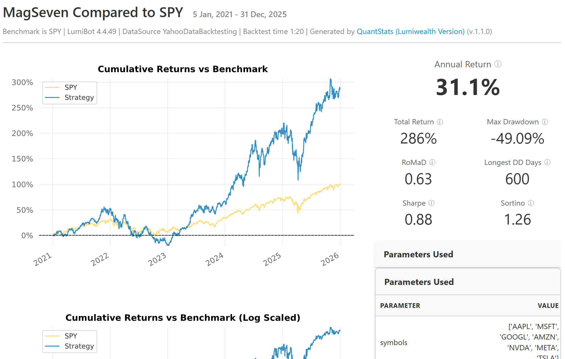
When the backtest completes, Lumibot generates a “tearsheet”–a standard industry report that aggregates performance metrics. Unlike the vectorized approach, this simulation accounted for the specific order execution logic defined in our class.

When moving to live trading (even with “Paper Money”) security is paramount. We use a .env file to store Alpaca credentials, ensuring they stay private and out of version control.

import os
from dotenv import load_dotenv
from lumibot.brokers import Alpaca
from lumibot.traders import Trader
from strategies.mag_seven import MagSeven

# Load .env file
load_dotenv()

# Parse Credentials
ALPACA_CREDS = {
    "API_KEY": os.getenv("ALPACA_API_KEY"),
    "API_SECRET": os.getenv("ALPACA_API_SECRET"),
    "PAPER": os.getenv("ALPACA_IS_PAPER", "True").lower() == "true",
}

if not ALPACA_CREDS["API_KEY"]:
    raise ValueError("Missing API Keys. Please check your .env file.")

# 1. Setup Broker
broker = Alpaca(ALPACA_CREDS)

# 2. Setup Strategy
strategy = MagSeven(broker=broker)

# 3. Run Trader
trader = Trader()
trader.add_strategy(strategy)

print("Starting Mag7 Bot... (Press Ctrl+C to stop)")
trader.run_all()

Running the bot for the first time is a fascinating experience.

There is a unique satisfaction in watching a terminal window wake up, connect to a broker across the world, and execute a complex basket trade that you researched and built from scratch.

Conclusion

At the end of this post, there is no secret formula to beat the market. In fact, it seems like finding real Alpha is incredibly difficult. The market is a highly efficient learning system; by the time a simple pattern like a “Golden Cross” is documented in a book, sophisticated institutions have likely already traded away the excess profit.

A boring, “Bogleheads” all-world ETF seems to be the most sound thing to do. But for the “fun” part–for experimenting and learning–we now have a professional laboratory.

A (hopefully valuable) outcome of this project is the infrastructure, aiming to enable a rigorous process. Most retail traders fail because they rely on intuition, visual patterns, and fragile setups. By building a professional-grade lab, we moved from guessing to engineering.

I have published the code for this entire setup–a Docker configuration, the VectorBT research notebooks, and the Lumibot execution scripts–as a template:

• algo-trading-template (GitHub)⤴ : If you have ever wanted to explore algorithmic trading but were intimidated by the technical overhead, this is for you.

This project was a one-week sprint into a very deep field, and there’s a lot that I wasn’t able to cover in this post. If you want to dive deeper into the mathematics of portfolio construction or the specifics of the libraries used, here are the best places to start:

• Efficient-Market Hypothesis (EMH)⤴ : The theory that asset prices reflect all available information. This explains why simple technical patterns (like our Moving Average crossover) are often “arbitraged away” and fail to generate consistent Alpha.
• Modern Portfolio Theory (MPT)⤴ : The mathematical framework for assembling a portfolio of assets such that the expected return is maximized for a given level of risk. This is the theoretical basis for the “Rebalancing” strategy we tested.
• VectorBT Documentation⤴ : The library used for our high-frequency backtesting. It is particularly powerful because it avoids slow Python loops by using NumPy broadcasting.
• Lumibot Documentation⤴ : The event-driven framework we used for the live bot. It handles the complexity of connecting to brokers like Alpaca or Interactive Brokers.
• PyPortfolioOpt⤴ : A fantastic library for financial portfolio optimization in Python. If you want to mathematically calculate the “Efficient Frontier” rather than just using equal weights (1/N), this is the industry standard tool.

Happy hunting.

Disclaimer: This article is for educational purposes only. Algorithmic trading involves significant risk of loss. Past performance is not indicative of future results. Never trade with money you cannot afford to lose.